58. The Income Fluctuation Problem II: Stochastic Returns on Assets#
In addition to what’s in Anaconda, this lecture will need the following libraries:
!pip install quantecon
58.1. Overview#
In this lecture, we continue our study of the income fluctuation problem.
While the interest rate was previously taken to be fixed, we now allow returns on assets to be state-dependent.
This matches the fact that most households with a positive level of assets face some capital income risk.
It has been argued that modeling capital income risk is essential for understanding the joint distribution of income and wealth (see, e.g., [Benhabib et al., 2015] or [Stachurski and Toda, 2019]).
Theoretical properties of the household savings model presented here are analyzed in detail in [Ma et al., 2020].
In terms of computation, we use a combination of time iteration and the endogenous grid method to solve the model quickly and accurately.
We require the following imports:
import matplotlib.pyplot as plt
import numpy as np
from numba import jit, float64
from numba.experimental import jitclass
from quantecon import MarkovChain
58.2. The Savings Problem#
In this section we review the household problem and optimality results.
58.2.1. Set Up#
A household chooses a consumption-asset path \(\{(c_t, a_t)\}\) to maximize
subject to
with initial condition \((a_0, Z_0)=(a,z)\) treated as given.
Note that \(\{R_t\}_{t \geq 1}\), the gross rate of return on wealth, is allowed to be stochastic.
The sequence \(\{Y_t \}_{t \geq 1}\) is non-financial income.
The stochastic components of the problem obey
where
the maps \(R\) and \(Y\) are time-invariant nonnegative functions,
the innovation processes \(\{\zeta_t\}\) and \(\{\eta_t\}\) are IID and independent of each other, and
\(\{Z_t\}_{t \geq 0}\) is an irreducible time-homogeneous Markov chain on a finite set \(\mathsf Z\)
Let \(P\) represent the Markov matrix for the chain \(\{Z_t\}_{t \geq 0}\).
Our assumptions on preferences are the same as our previous lecture on the income fluctuation problem.
As before, \(\mathbb E_z \hat X\) means expectation of next period value \(\hat X\) given current value \(Z = z\).
58.2.2. Assumptions#
We need restrictions to ensure that the objective (58.1) is finite and the solution methods described below converge.
We also need to ensure that the present discounted value of wealth does not grow too quickly.
When \(\{R_t\}\) was constant we required that \(\beta R < 1\).
Since it is now stochastic, we require that
Notice that, when \(\{R_t\}\) takes some constant value \(R\), this reduces to the previous restriction \(\beta R < 1\).
The value \(G_R\) can be thought of as the long run (geometric) average gross rate of return.
More intuition behind (58.4) is provided in [Ma et al., 2020].
Discussion on how to check it is given below.
Finally, we impose some routine technical restrictions on non-financial income.
One relatively simple setting where all these restrictions are satisfied is the IID and CRRA environment of [Benhabib et al., 2015].
58.2.3. Optimality#
Let the class of candidate consumption policies \(\mathscr C\) be defined as before.
In [Ma et al., 2020] it is shown that, under the stated assumptions,
any \(\sigma \in \mathscr C\) satisfying the Euler equation is an optimal policy and
exactly one such policy exists in \(\mathscr C\).
In the present setting, the Euler equation takes the form
(Intuition and derivation are similar to our earlier lecture on the income fluctuation problem.)
We again solve the Euler equation using time iteration, iterating with a Coleman–Reffett operator \(K\) defined to match the Euler equation (58.5).
58.3. Solution Algorithm#
58.3.1. A Time Iteration Operator#
Our definition of the candidate class \(\sigma \in \mathscr C\) of consumption policies is the same as in our earlier lecture on the income fluctuation problem.
For fixed \(\sigma \in \mathscr C\) and \((a,z) \in \mathbf S\), the value \(K\sigma(a,z)\) of the function \(K\sigma\) at \((a,z)\) is defined as the \(\xi \in (0,a]\) that solves
The idea behind \(K\) is that, as can be seen from the definitions, \(\sigma \in \mathscr C\) satisfies the Euler equation if and only if \(K\sigma(a, z) = \sigma(a, z)\) for all \((a, z) \in \mathbf S\).
This means that fixed points of \(K\) in \(\mathscr C\) and optimal consumption policies exactly coincide (see [Ma et al., 2020] for more details).
58.3.2. Convergence Properties#
As before, we pair \(\mathscr C\) with the distance
It can be shown that
\((\mathscr C, \rho)\) is a complete metric space,
there exists an integer \(n\) such that \(K^n\) is a contraction mapping on \((\mathscr C, \rho)\), and
The unique fixed point of \(K\) in \(\mathscr C\) is the unique optimal policy in \(\mathscr C\).
We now have a clear path to successfully approximating the optimal policy: choose some \(\sigma \in \mathscr C\) and then iterate with \(K\) until convergence (as measured by the distance \(\rho\)).
58.3.3. Using an Endogenous Grid#
In the study of that model we found that it was possible to further accelerate time iteration via the endogenous grid method.
We will use the same method here.
The methodology is the same as it was for the optimal growth model, with the minor exception that we need to remember that consumption is not always interior.
In particular, optimal consumption can be equal to assets when the level of assets is low.
58.3.3.1. Finding Optimal Consumption#
The endogenous grid method (EGM) calls for us to take a grid of savings values \(s_i\), where each such \(s\) is interpreted as \(s = a - c\).
For the lowest grid point we take \(s_0 = 0\).
For the corresponding \(a_0, c_0\) pair we have \(a_0 = c_0\).
This happens close to the origin, where assets are low and the household consumes all that it can.
Although there are many solutions, the one we take is \(a_0 = c_0 = 0\), which pins down the policy at the origin, aiding interpolation.
For \(s > 0\), we have, by definition, \(c < a\), and hence consumption is interior.
Hence the max component of (58.5) drops out, and we solve for
at each \(s_i\).
58.3.3.2. Iterating#
Once we have the pairs \(\{s_i, c_i\}\), the endogenous asset grid is obtained by \(a_i = c_i + s_i\).
Also, we held \(z \in \mathsf Z\) in the discussion above so we can pair it with \(a_i\).
An approximation of the policy \((a, z) \mapsto \sigma(a, z)\) can be obtained by interpolating \(\{a_i, c_i\}\) at each \(z\).
In what follows, we use linear interpolation.
58.3.4. Testing the Assumptions#
Convergence of time iteration is dependent on the condition \(\beta G_R < 1\) being satisfied.
One can check this using the fact that \(G_R\) is equal to the spectral radius of the matrix \(L\) defined by
This identity is proved in [Ma et al., 2020], where \(\phi\) is the density of the innovation \(\zeta_t\) to returns on assets.
(Remember that \(\mathsf Z\) is a finite set, so this expression defines a matrix.)
Checking the condition is even easier when \(\{R_t\}\) is IID.
In that case, it is clear from the definition of \(G_R\) that \(G_R\) is just \(\mathbb E R_t\).
We test the condition \(\beta \mathbb E R_t < 1\) in the code below.
58.4. Numba Implementation#
We will assume that \(R_t = \exp(a_r \zeta_t + b_r)\) where \(a_r, b_r\) are constants and \(\{ \zeta_t\}\) is IID standard normal.
We allow labor income to be correlated, with
where \(\{ \eta_t\}\) is also IID standard normal and \(\{ Z_t\}\) is a Markov chain taking values in \(\{0, 1\}\).
ifp_data = [
    ('γ', float64),              # utility parameter
    ('β', float64),              # discount factor
    ('P', float64[:, :]),        # transition probs for z_t
    ('a_r', float64),            # scale parameter for R_t
    ('b_r', float64),            # additive parameter for R_t
    ('a_y', float64),            # scale parameter for Y_t
    ('b_y', float64),            # additive parameter for Y_t
    ('s_grid', float64[:]),      # Grid over savings
    ('η_draws', float64[:]),     # Draws of innovation η for MC
    ('ζ_draws', float64[:])      # Draws of innovation ζ for MC
]
@jitclass(ifp_data)
class IFP:
    """
    A class that stores primitives for the income fluctuation
    problem.
    """

    def __init__(self,
                 γ=1.5,
                 β=0.96,
                 P=np.array([(0.9, 0.1),
                             (0.1, 0.9)]),
                 a_r=0.1,
                 b_r=0.0,
                 a_y=0.2,
                 b_y=0.5,
                 shock_draw_size=50,
                 grid_max=10,
                 grid_size=100,
                 seed=1234):

        np.random.seed(seed)  # arbitrary seed

        self.P, self.γ, self.β = P, γ, β
        self.a_r, self.b_r, self.a_y, self.b_y = a_r, b_r, a_y, b_y
        self.η_draws = np.random.randn(shock_draw_size)
        self.ζ_draws = np.random.randn(shock_draw_size)
        self.s_grid = np.linspace(0, grid_max, grid_size)

        # Test stability assuming {R_t} is IID and adopts the lognormal
        # specification given below.  The test is then β E R_t < 1.
        ER = np.exp(b_r + a_r**2 / 2)
        assert β * ER < 1, "Stability condition failed."

    # Marginal utility
    def u_prime(self, c):
        return c**(-self.γ)

    # Inverse of marginal utility
    def u_prime_inv(self, c):
        return c**(-1/self.γ)

    def R(self, z, ζ):
        return np.exp(self.a_r * ζ + self.b_r)

    def Y(self, z, η):
        return np.exp(self.a_y * η + (z * self.b_y))
Here’s the Coleman-Reffett operator based on EGM:
58.4.1. Implementation Details#
The implementation of operator \(K\) maps directly to equation (58.6).
The left side \(u'(\xi)\) becomes u_prime_inv(β * Ez) after solving for \(\xi\).
The expectation term \(\mathbb E_z \hat{R} (u' \circ \sigma)[\hat{R}(a - \xi) + \hat{Y}, \hat{Z}]\) is computed via Monte Carlo averaging over future states and shocks.
The max with \(u'(a)\) is handled implicitly—the endogenous grid method naturally handles the liquidity constraint since we only solve for interior consumption where \(c < a\).
@jit
def K(ae_vals, c_vals, ifp):
    """
    The Coleman--Reffett operator for the income fluctuation problem,
    using the endogenous grid method.

        * ifp is an instance of IFP
        * ae_vals[i, z] is an asset grid
        * c_vals[i, z] is consumption at ae_vals[i, z]
    """

    # Simplify names
    u_prime, u_prime_inv = ifp.u_prime, ifp.u_prime_inv
    R, Y, P, β = ifp.R, ifp.Y, ifp.P, ifp.β
    s_grid, η_draws, ζ_draws = ifp.s_grid, ifp.η_draws, ifp.ζ_draws
    n = len(P)

    # Create consumption function by linear interpolation
    σ = lambda a, z: np.interp(a, ae_vals[:, z], c_vals[:, z])

    # Allocate memory
    c_out = np.empty_like(c_vals)

    # Obtain c_i at each s_i, z, store in c_out[i, z], computing
    # the expectation term by Monte Carlo
    for i, s in enumerate(s_grid):
        for z in range(n):
            # Compute expectation
            Ez = 0.0
            for z_hat in range(n):
                for η in ifp.η_draws:
                    for ζ in ifp.ζ_draws:
                        R_hat = R(z_hat, ζ)
                        Y_hat = Y(z_hat, η)
                        U = u_prime(σ(R_hat * s + Y_hat, z_hat))
                        Ez += R_hat * U * P[z, z_hat]
            Ez = Ez / (len(η_draws) * len(ζ_draws))
            c_out[i, z] =  u_prime_inv(β * Ez)

    # Calculate endogenous asset grid
    ae_out = np.empty_like(c_out)
    for z in range(n):
        ae_out[:, z] = s_grid + c_out[:, z]

    # Fixing a consumption-asset pair at (0, 0) improves interpolation
    c_out[0, :] = 0
    ae_out[0, :] = 0

    return ae_out, c_out
58.4.2. Code Walkthrough#
The operator creates a consumption function σ by interpolating the input policy, then uses triple nested loops to compute the expectation via Monte Carlo averaging over savings grid points, current states, future states, and shock realizations.
After computing optimal consumption \(c_i\) at each savings level \(s_i\) by inverting marginal utility, we construct the endogenous asset grid using \(a_i = s_i + c_i\).
Setting consumption and assets to zero at the origin ensures smooth interpolation near zero assets, where the household consumes everything.
The next function solves for an approximation of the optimal consumption policy via time iteration.
def solve_model_time_iter(model,        # Class with model information
                          a_vec,        # Initial condition for assets
                          σ_vec,        # Initial condition for consumption
                          tol=1e-4,
                          max_iter=1000,
                          verbose=True,
                          print_skip=25):

    # Set up loop
    i = 0
    error = tol + 1

    while i < max_iter and error > tol:
        a_new, σ_new = K(a_vec, σ_vec, model)
        error = np.max(np.abs(σ_vec - σ_new))
        i += 1
        if verbose and i % print_skip == 0:
            print(f"Error at iteration {i} is {error}.")
        a_vec, σ_vec = np.copy(a_new), np.copy(σ_new)

    if error > tol:
        print("Failed to converge!")
    elif verbose:
        print(f"\nConverged in {i} iterations.")

    return a_new, σ_new
This function implements fixed-point iteration by repeatedly applying the operator \(K\) until the policy converges.
Convergence is measured by the maximum absolute change in consumption across all states.
The operator is guaranteed to converge due to the contraction property discussed earlier.
Now we are ready to create an instance at the default parameters.
ifp = IFP()
The default parameters represent a calibration with moderate risk aversion (\(\gamma = 1.5\), CRRA utility) and a quarterly discount factor (\(\beta = 0.96\), corresponding to roughly 4% annual discounting).
The Markov chain has high persistence (90% probability of staying in the current state), while returns have 10% volatility around a zero mean log return (\(a_r = 0.1\), \(b_r = 0.0\)).
Labor income is state-dependent: \(Y_t = \exp(0.2 \eta_t + 0.5 Z_t)\) implies higher expected income in the good state (\(Z_t = 1\)) compared to the bad state (\(Z_t = 0\)).
Next we set up an initial condition, which corresponds to consuming all assets.
# Initial guess of σ = consume all assets
k = len(ifp.s_grid)
n = len(ifp.P)
σ_init = np.empty((k, n))
for z in range(n):
    σ_init[:, z] = ifp.s_grid
a_init = np.copy(σ_init)
Let’s generate an approximation solution.
a_star, σ_star = solve_model_time_iter(ifp, a_init, σ_init, print_skip=5)
Error at iteration 5 is 0.5081944529506552.
Error at iteration 10 is 0.1057246950930697.
Error at iteration 15 is 0.03658262202883744.
Error at iteration 20 is 0.013936729965906114.
Error at iteration 25 is 0.00529216526971199.
Error at iteration 30 is 0.0019748126990770665.
Error at iteration 35 is 0.0007219210463285108.
Error at iteration 40 is 0.0002590544496094971.
Error at iteration 45 is 9.163966595471251e-05.

Converged in 45 iterations.
Here’s a plot of the resulting consumption policy.
fig, ax = plt.subplots()
for z in range(len(ifp.P)):
    ax.plot(a_star[:, z], σ_star[:, z], label=f"consumption when $z={z}$")

plt.legend()
plt.show()
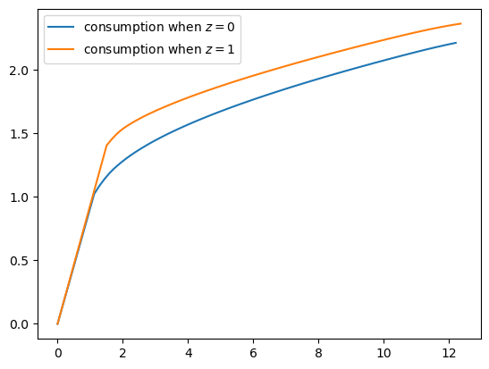
Notice that we consume all assets in the lower range of the asset space.
This is because we anticipate income \(Y_{t+1}\) tomorrow, which makes the need to save less urgent.
Observe that consuming all assets ends earlier (at lower asset levels) when \(z=0\) compared to \(z=1\).
This occurs because expected future income is lower in the bad state (\(z=0\)), so the household begins precautionary saving at lower wealth levels.
In contrast, when \(z=1\) (good state), higher expected future income allows the household to consume all assets up to a higher threshold before savings become optimal.
58.4.3. Law of Motion#
Let’s try to get some idea of what will happen to assets over the long run under this consumption policy.
As with our earlier lecture on the income fluctuation problem, we begin by producing a 45 degree diagram showing the law of motion for assets
# Good and bad state mean labor income
Y_mean = [np.mean(ifp.Y(z, ifp.η_draws)) for z in (0, 1)]
# Mean returns
R_mean = np.mean(ifp.R(z, ifp.ζ_draws))

a = a_star
fig, ax = plt.subplots()
for z, lb in zip((0, 1), ('bad state', 'good state')):
    ax.plot(a[:, z], R_mean * (a[:, z] - σ_star[:, z]) + Y_mean[z] , label=lb)

ax.plot(a[:, 0], a[:, 0], 'k--')
ax.set(xlabel='current assets', ylabel='next period assets')

ax.legend()
plt.show()
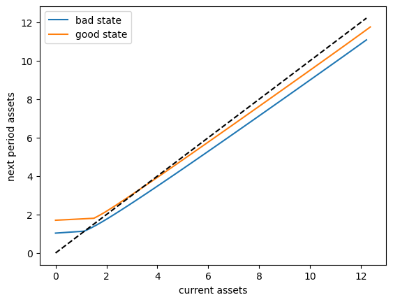
The unbroken lines represent, for each \(z\), an average update function for assets, given by
Here
\(\bar R = \mathbb E R_t\), which is mean returns and
\(\bar Y(z) = \mathbb E_z Y(z, \eta_t)\), which is mean labor income in state \(z\).
The dashed line is the 45 degree line.
We can see from the figure that the dynamics will be stable — assets do not diverge even in the highest state.
58.5. JAX Implementation#
We now provide a JAX implementation of the model.
JAX is a high-performance numerical computing library that provides automatic differentiation and JIT compilation, with support for GPU/TPU acceleration.
First we need to import JAX and related libraries:
import jax
import jax.numpy as jnp
from jax import vmap
from typing import NamedTuple

# Import jax.jit with a different name to avoid conflict with numba.jit
jax_jit = jax.jit
We enable 64-bit precision in JAX to ensure accurate results that match the Numba implementation:
jax.config.update("jax_enable_x64", True)
Here’s the JAX version of the IFP class using NamedTuple for compatibility with JAX’s JIT compilation:
class IFP_JAX(NamedTuple):
    """
    A NamedTuple that stores primitives for the income fluctuation
    problem, using JAX.
    """
    γ: float
    β: float
    P: jnp.ndarray
    a_r: float
    b_r: float
    a_y: float
    b_y: float
    s_grid: jnp.ndarray
    η_draws: jnp.ndarray
    ζ_draws: jnp.ndarray


def create_ifp_jax(γ=1.5,
                   β=0.96,
                   P=np.array([(0.9, 0.1),
                               (0.1, 0.9)]),
                   a_r=0.1,
                   b_r=0.0,
                   a_y=0.2,
                   b_y=0.5,
                   shock_draw_size=50,
                   grid_max=10,
                   grid_size=100,
                   seed=1234):
    """
    Create an instance of IFP_JAX with the given parameters.
    """
    # Test stability assuming {R_t} is IID and adopts the lognormal
    # specification given below.  The test is then β E R_t < 1.
    ER = np.exp(b_r + a_r**2 / 2)
    assert β * ER < 1, "Stability condition failed."

    # Convert to JAX arrays
    P_jax = jnp.array(P)

    # Generate random draws using JAX
    key = jax.random.PRNGKey(seed)
    key, subkey1, subkey2 = jax.random.split(key, 3)
    η_draws = jax.random.normal(subkey1, (shock_draw_size,))
    ζ_draws = jax.random.normal(subkey2, (shock_draw_size,))
    s_grid = jnp.linspace(0, grid_max, grid_size)

    return IFP_JAX(γ=γ, β=β, P=P_jax, a_r=a_r, b_r=b_r, a_y=a_y, b_y=b_y,
                   s_grid=s_grid, η_draws=η_draws, ζ_draws=ζ_draws)


# Utility functions for the IFP model

def u_prime(c, γ):
    """Marginal utility"""
    return c**(-γ)

def u_prime_inv(c, γ):
    """Inverse of marginal utility"""
    return c**(-1/γ)

def R(z, ζ, a_r, b_r):
    """Gross return on assets"""
    return jnp.exp(a_r * ζ + b_r)

def Y(z, η, a_y, b_y):
    """Labor income"""
    return jnp.exp(a_y * η + (z * b_y))
Here’s the Coleman-Reffett operator using JAX:
@jax_jit
def K_jax(ae_vals, c_vals, ifp):
    """
    The Coleman--Reffett operator for the income fluctuation problem,
    using the endogenous grid method with JAX.

        * ifp is an instance of IFP_JAX
        * ae_vals[i, z] is an asset grid
        * c_vals[i, z] is consumption at ae_vals[i, z]
    """

    # Extract parameters from ifp
    γ, β, P = ifp.γ, ifp.β, ifp.P
    a_r, b_r, a_y, b_y = ifp.a_r, ifp.b_r, ifp.a_y, ifp.b_y
    s_grid, η_draws, ζ_draws = ifp.s_grid, ifp.η_draws, ifp.ζ_draws
    n = len(P)

    # Allocate memory
    c_out = jnp.empty_like(c_vals)

    # Obtain c_i at each s_i, z, store in c_out[i, z], computing
    # the expectation term by Monte Carlo
    def compute_expectation(s, z):
        """Compute expectation for given s and z"""
        def inner_expectation(z_hat):
            # Vectorize over shocks
            def compute_term(η, ζ):
                R_hat = R(z_hat, ζ, a_r, b_r)
                Y_hat = Y(z_hat, η, a_y, b_y)
                a_val = R_hat * s + Y_hat
                # Interpolate consumption
                c_interp = jnp.interp(a_val, ae_vals[:, z_hat], c_vals[:, z_hat])
                U = u_prime(c_interp, γ)
                return R_hat * U

            # Vectorize over all shock combinations
            η_grid, ζ_grid = jnp.meshgrid(η_draws, ζ_draws, indexing='ij')
            terms = vmap(vmap(compute_term))(η_grid, ζ_grid)
            return P[z, z_hat] * jnp.mean(terms)

        # Sum over z_hat states
        Ez = jnp.sum(vmap(inner_expectation)(jnp.arange(n)))
        return u_prime_inv(β * Ez, γ)

    # Vectorize over s_grid and z
    c_out = vmap(vmap(compute_expectation, in_axes=(None, 0)),
                  in_axes=(0, None))(s_grid, jnp.arange(n))

    # Calculate endogenous asset grid
    ae_out = s_grid[:, None] + c_out

    # Fixing a consumption-asset pair at (0, 0) improves interpolation
    c_out = c_out.at[0, :].set(0)
    ae_out = ae_out.at[0, :].set(0)

    return ae_out, c_out
The next function solves for an approximation of the optimal consumption policy via time iteration using JAX:
def solve_model_time_iter_jax(model,        # Class with model information
                               a_vec,        # Initial condition for assets
                               σ_vec,        # Initial condition for consumption
                               tol=1e-4,
                               max_iter=1000,
                               verbose=True,
                               print_skip=25):

    # Set up loop
    i = 0
    error = tol + 1

    while i < max_iter and error > tol:
        a_new, σ_new = K_jax(a_vec, σ_vec, model)
        error = jnp.max(jnp.abs(σ_vec - σ_new))
        i += 1
        if verbose and i % print_skip == 0:
            print(f"Error at iteration {i} is {error}.")
        a_vec, σ_vec = a_new, σ_new

    if error > tol:
        print("Failed to converge!")
    elif verbose:
        print(f"\nConverged in {i} iterations.")

    return a_new, σ_new
Now we can create an instance and solve the model using JAX:
ifp_jax = create_ifp_jax()
Set up the initial condition:
# Initial guess of σ = consume all assets
k = len(ifp_jax.s_grid)
n = len(ifp_jax.P)
σ_init_jax = jnp.empty((k, n))
for z in range(n):
    σ_init_jax = σ_init_jax.at[:, z].set(ifp_jax.s_grid)
a_init_jax = σ_init_jax.copy()
Let’s generate an approximation solution with JAX:
a_star_jax, σ_star_jax = solve_model_time_iter_jax(ifp_jax, a_init_jax, σ_init_jax, print_skip=5)
Error at iteration 5 is 0.5056668931888328.
Error at iteration 10 is 0.1034861379984835.
Error at iteration 15 is 0.03412817463153939.
Error at iteration 20 is 0.01201705155740429.
Error at iteration 25 is 0.004145424467285608.
Error at iteration 30 is 0.001391633566658168.
Error at iteration 35 is 0.0004556358742306976.
Error at iteration 40 is 0.00014622723914969882.

Converged in 42 iterations.
Here’s a plot comparing the JAX solution with the Numba solution:
fig, ax = plt.subplots()
for z in range(len(ifp_jax.P)):
    ax.plot(np.array(a_star_jax[:, z]), np.array(σ_star_jax[:, z]),
            label=f"JAX: consumption when $z={z}$", linestyle='--')
    ax.plot(a_star[:, z], σ_star[:, z],
            label=f"Numba: consumption when $z={z}$", linestyle='-', alpha=0.6)

plt.legend()
plt.show()
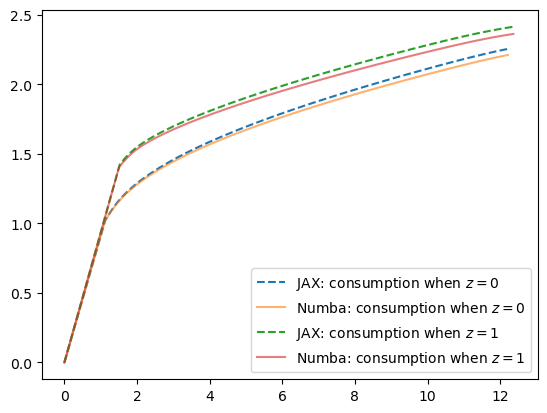
58.5.1. Comparison of Numba and JAX Solutions#
Now let’s verify that both implementations produce nearly identical results.
With 64-bit precision enabled in JAX, we expect the solutions to be very close.
Let’s compute the maximum absolute differences:
# Convert JAX arrays to NumPy for comparison
a_star_jax_np = np.array(a_star_jax)
σ_star_jax_np = np.array(σ_star_jax)

# Compute differences
a_diff = np.abs(a_star - a_star_jax_np)
σ_diff = np.abs(σ_star - σ_star_jax_np)

print("Comparison of Numba and JAX solutions:")
print("=" * 50)
print(f"Max absolute difference in asset grid: {np.max(a_diff):.3e}")
print(f"Mean absolute difference in asset grid: {np.mean(a_diff):.3e}")
print(f"Max absolute difference in consumption: {np.max(σ_diff):.3e}")
print(f"Mean absolute difference in consumption: {np.mean(σ_diff):.3e}")
Comparison of Numba and JAX solutions:
==================================================
Max absolute difference in asset grid: 5.377e-02
Mean absolute difference in asset grid: 3.559e-02
Max absolute difference in consumption: 5.377e-02
Mean absolute difference in consumption: 3.559e-02
Let’s also visualize the differences:
fig, axes = plt.subplots(1, 2, figsize=(12, 4))

for z in range(len(ifp.P)):
    axes[0].plot(a_star[:, z], a_diff[:, z], label=f'z={z}')
    axes[1].plot(a_star[:, z], σ_diff[:, z], label=f'z={z}')

axes[0].set_xlabel('assets')
axes[0].set_ylabel('absolute difference')
axes[0].set_title('Asset Grid Differences: |Numba - JAX|')
axes[0].legend()

axes[1].set_xlabel('assets')
axes[1].set_ylabel('absolute difference')
axes[1].set_title('Consumption Differences: |Numba - JAX|')
axes[1].legend()

plt.tight_layout()
plt.show()
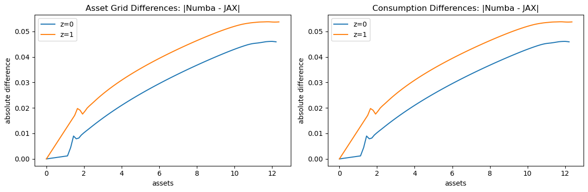
As we can see, the differences between the two implementations are extremely small (on the order of machine precision), confirming that both methods produce essentially identical results.
The tiny differences arise from:
Different random number generators (NumPy vs JAX)
Minor differences in floating-point operations order
Different interpolation implementations
Despite these minor numerical differences, both implementations converge to the same optimal policy.
The JAX implementation provides several advantages:
GPU/TPU acceleration: JAX can automatically utilize GPU/TPU hardware for faster computation
Automatic differentiation: JAX provides automatic differentiation, which can be useful for sensitivity analysis
Functional programming: JAX encourages a functional style that can be easier to reason about and parallelize
58.6. Exercises#
Exercise 58.1
Let’s repeat our earlier exercise on the long-run cross sectional distribution of assets.
In that exercise, we used a relatively simple income fluctuation model.
In the solution, we found the shape of the asset distribution to be unrealistic.
In particular, we failed to match the long right tail of the wealth distribution.
Your task is to try again, repeating the exercise, but now with our more sophisticated model.
Use the default parameters.
Solution
First we write a function to compute a long asset series.
Because we want to JIT-compile the function, we code the solution in a way that breaks some rules on good programming style.
For example, we will pass in the solutions a_star, σ_star along with
ifp, even though it would be more natural to just pass in ifp and then
solve inside the function.
The reason we do this is that solve_model_time_iter is not
JIT-compiled.
@jit
def compute_asset_series(ifp, a_star, σ_star, z_seq, T=500_000):
    """
    Simulates a time series of length T for assets, given optimal
    savings behavior.

        * ifp is an instance of IFP
        * a_star is the endogenous grid solution
        * σ_star is optimal consumption on the grid
        * z_seq is a time path for {Z_t}

    """

    # Create consumption function by linear interpolation
    σ = lambda a, z: np.interp(a, a_star[:, z], σ_star[:, z])

    # Simulate the asset path
    a = np.zeros(T+1)
    for t in range(T):
        z = z_seq[t]
        ζ, η = np.random.randn(), np.random.randn()
        R = ifp.R(z, ζ)
        Y = ifp.Y(z, η)
        a[t+1] = R * (a[t] - σ(a[t], z)) + Y
    return a
Now we call the function, generate the series and then histogram it, using the solutions computed above.
T = 1_000_000
mc = MarkovChain(ifp.P)
z_seq = mc.simulate(T, random_state=1234)

a = compute_asset_series(ifp, a_star, σ_star, z_seq, T=T)

fig, ax = plt.subplots()
ax.hist(a, bins=40, alpha=0.5, density=True)
ax.set(xlabel='assets')
plt.show()
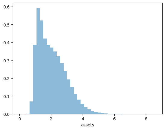
Now we have managed to successfully replicate the long right tail of the wealth distribution.
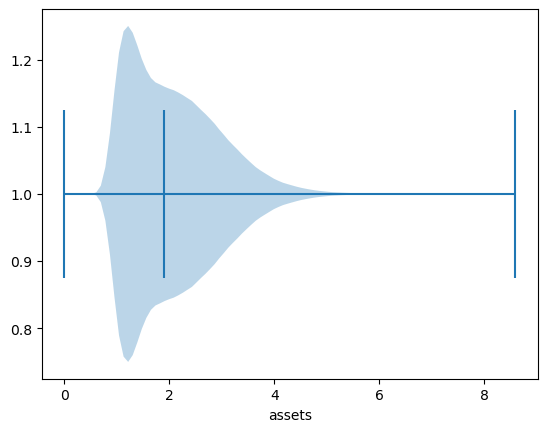
Here’s another view of this using a horizontal violin plot.
fig, ax = plt.subplots()
ax.violinplot(a, vert=False, showmedians=True)
ax.set(xlabel='assets')
plt.show()