45. Job Search IV: Fitted Value Function Iteration#
45.1. Overview#
This lecture follows on from the job search model with separation presented in the previous lecture.
That lecture combined exogenous job separation events and a Markov wage offer process.
In this lecture we continue with this set and, in addition, allow the wage offer process to be continuous rather than discrete.
In particular,
and \(\{Z_t\}\) is IID and standard normal.
While we already considered continuous wage distributions briefly in Job Search I: The McCall Search Model, the change was relatively trivial in that case.
The reason is that we were able to reduce the problem to solving for a single scalar value (the continuation value).
Here, in our Markov setting, the change is less trivial, since a continuous wage distribution leads to an uncountably infinite state space.
The infinite state space leads to additional challenges, particularly when it comes to applying value function iteration (VFI).
These challenges will lead us to modify VFI by adding an interpolation step.
The combination of VFI and this interpolation step is called fitted value function iteration (fitted VFI).
Fitted VFI is very common in practice, so we will take some time to work through the details.
In addition to what’s in Anaconda, this lecture will need the following libraries
!pip install quantecon jax
We will use the following imports:
import matplotlib.pyplot as plt
import jax
import jax.numpy as jnp
from jax import lax
from typing import NamedTuple
from functools import partial
import quantecon as qe
45.2. Model#
Assuming that readers are familiar with the content of Job Search III: Search with Separation and Markov Wages, the model can be summarized as follows.
Wage offers follow a continuous Markov process: \(W_t = \exp(X_t)\) where \(X_{t+1} = \rho X_t + \nu Z_{t+1}\)
\(\{Z_t\}\) is IID and standard normal
Jobs terminate with probability \(\alpha\) each period (separation rate)
Unemployed workers receive compensation \(c\) per period
Workers have CRRA utility \(u(x) = \frac{x^{1-\gamma} - 1}{1-\gamma}\)
Future payoffs are discounted by factor \(\beta \in (0,1)\)
45.3. Solution method#
Let’s discuss how we can solve this model.
The only real change from Job Search III: Search with Separation and Markov Wages is that we replace sums with integrals.
45.3.1. Value function iteration#
In the discrete case, we ended up iterating on the Bellman operator
where
Here we iterate on the same law after changing the definition of the \(P\) operator to
where \(p(w, \cdot)\) is the conditional density of \(w'\) given \(w\).
Here we are thinking of \(v_u\) as a function on all of \(\mathbb{R}_+\).
After taking \(\psi\) to be the standard normal density, we can write the expression above more explicitly as
To understand this expression, recall that \(W_t = \exp(X_t)\) where \(X_{t+1} = \rho X_t + \nu Z_{t+1}\).
As a result \(W_{t+1} = \exp(X_{t+1}) = \exp(\rho \log(W_t) + \nu Z_{t+1}) = W_t^\rho \exp(\nu Z_{t+1})\).
The integral above regards the current wage \(W_t\) as fixed at \(w\) and takes the expectation of \(v_u(w^\rho \exp(\nu Z_{t+1}))\).
45.3.2. Fitting#
In theory, we should now proceed as follows:
Begin with a guess \(v\)
Applying \(T\) to obtain the update \(v' = Tv\)
Unless some stopping condition is satisfied, set \(v = v'\) and go to step 2.
However, there is a problem we must confront before we implement this procedure: The iterates of the value function can neither be calculated exactly nor stored on a computer.
To see the issue, consider (45.1).
Even if \(v\) is a known function, the only way to store its update \(v'\) is to record its value \(v'(w)\) for every \(w \in \mathbb R_+\).
Clearly, this is impossible.
45.3.3. Fitted value function iteration#
What we will do instead is use fitted value function iteration.
The procedure is as follows:
Let a current guess \(v\) be given.
Now we record the value of the function \(v'\) at only finitely many “grid” points \(w_1 < w_2 < \cdots < w_I\) and then reconstruct \(v'\) from this information when required.
More precisely, the algorithm will be
Begin with an array \(\mathbf v\) representing the values of an initial guess of the value function on some grid points \(\{w_i\}\).
Build a function \(v\) on the state space \(\mathbb R_+\) by interpolation or approximation, based on \(\mathbf v\) and \(\{ w_i\}\).
Obtain and record the samples of the updated function \(v'(w_i)\) on each grid point \(w_i\).
Unless some stopping condition is satisfied, take this as the new array and go to step 1.
How should we go about step 2?
This is a problem of function approximation, and there are many ways to approach it.
What’s important here is that the function approximation scheme must not only produce a good approximation to each \(v\), but also that it combines well with the broader iteration algorithm described above.
One good choice from both respects is continuous piecewise linear interpolation.
This method
combines well with value function iteration (see, e.g., [Gordon, 1995] or [Stachurski, 2008]) and
preserves useful shape properties such as monotonicity and concavity/convexity.
Linear interpolation will be implemented using JAX’s interpolation function jnp.interp.
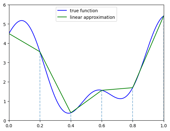
The next figure illustrates piecewise linear interpolation of an arbitrary function on grid points \(0, 0.2, 0.4, 0.6, 0.8, 1\).
def f(x):
    y1 = 2 * jnp.cos(6 * x) + jnp.sin(14 * x)
    return y1 + 2.5

c_grid = jnp.linspace(0, 1, 6)
f_grid = jnp.linspace(0, 1, 150)

def Af(x):
    return jnp.interp(x, c_grid, f(c_grid))

fig, ax = plt.subplots()

ax.plot(f_grid, f(f_grid), 'b-', label='true function')
ax.plot(f_grid, Af(f_grid), 'g-', label='linear approximation')
ax.vlines(c_grid, c_grid * 0, f(c_grid), linestyle='dashed', alpha=0.5)

ax.legend(loc="upper center")

ax.set(xlim=(0, 1), ylim=(0, 6))
plt.show()
45.4. Implementation#
Let’s code up and solve the model.
45.4.1. Setup#
The first step is to build a JAX-compatible structure for the McCall model with separation and a continuous wage offer distribution.
The key computational challenge is evaluating the conditional expectation \((Pv_u)(w) = \int v_u(w') p(w, w') dw'\) at each wage grid point.
Recall that we have:
where \(\psi\) is the standard normal density.
We will approximate this integral using Monte Carlo integration with draws \(\{Z_i\}\) from the standard normal distribution:
For this reason, our data structure will include a fixed set of IID \(N(0,1)\) draws \(\{Z_i\}\).
class Model(NamedTuple):
    c: float              # unemployment compensation
    α: float              # job separation rate
    β: float              # discount factor
    ρ: float              # wage persistence
    ν: float              # wage volatility
    γ: float              # utility parameter
    w_grid: jnp.ndarray   # grid of points for fitted VFI
    z_draws: jnp.ndarray  # draws from the standard normal distribution

def create_mccall_model(
        c: float = 1.0,
        α: float = 0.1,
        β: float = 0.96,
        ρ: float = 0.9,
        ν: float = 0.2,
        γ: float = 1.5,
        grid_size: int = 100,
        mc_size: int = 1000,
        seed: int = 1234
    ):
    """Factory function to create a McCall model instance."""

    key = jax.random.PRNGKey(seed)
    z_draws = jax.random.normal(key, (mc_size,))

    # Discretize just to get a suitable wage grid for interpolation
    mc = qe.markov.tauchen(grid_size, ρ, ν)
    w_grid = jnp.exp(jnp.array(mc.state_values))

    return Model(c, α, β, ρ, ν, γ, w_grid, z_draws)
We use the same CRRA utility function as in the discrete case:
def u(x, γ):
    return (x**(1 - γ) - 1) / (1 - γ)
45.4.2. Iteration#
Here is the Bellman operator, where we use Monte Carlo integration to evaluate the expectation.
def T(model, v):
    """Update the value function."""

    # Unpack model parameters
    c, α, β, ρ, ν, γ, w_grid, z_draws = model

    # Interpolate array represented value function
    vf = lambda x: jnp.interp(x, w_grid, v)

    def compute_expectation(w):
        # Use Monte Carlo to evaluate integral (P v)(w) = E[v(W' | w)]
        # where W' = w^ρ * exp(ν * Z)
        w_next = w**ρ * jnp.exp(ν * z_draws)
        return jnp.mean(vf(w_next))

    compute_exp_on_grid = jax.vmap(compute_expectation)
    Pv = compute_exp_on_grid(w_grid)

    d = 1 / (1 - β * (1 - α))
    v_e = d * (u(w_grid, γ) + α * β * Pv)
    continuation_values = u(c, γ) + β * Pv
    return jnp.maximum(v_e, continuation_values)
Here’s the solver, which computes an approximate fixed point \(v_u\) of \(T\).
@jax.jit
def vfi(
        model: Model,
        tolerance: float = 1e-6,   # Error tolerance
        max_iter: int = 100_000,   # Max iteration bound
    ):
    """
    Compute the fixed point v_u of T.

    """

    v_init = jnp.zeros(model.w_grid.shape)

    def cond(loop_state):
        v, error, i = loop_state
        return (error > tolerance) & (i <= max_iter)

    def update(loop_state):
        v, error, i = loop_state
        v_new = T(model, v)
        error = jnp.max(jnp.abs(v_new - v))
        new_loop_state = v_new, error, i + 1
        return new_loop_state

    initial_state = (v_init, tolerance + 1, 1)
    final_loop_state = lax.while_loop(cond, update, initial_state)
    v_final, error, i = final_loop_state

    return v_final
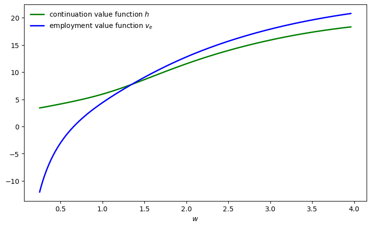
Here’s a function that uses a solution \(v_u\) to compute the remaining functions of interest: \(v_u\), and the continuation value function \(h\).
We use the same expressions as we did in the discrete case, after replacing sums with integrals.
def compute_solution_functions(model, v_u):

    # Interpolate v_u
    vf = lambda x: jnp.interp(x, w_grid, v_u)

    def compute_expectation(w):
        # Use Monte Carlo to evaluate integral (P v)(w)
        # Compute E[v(w' | w)] where w' = w^ρ * exp(ν * z)
        w_next = w**ρ * jnp.exp(ν * z_draws)
        return jnp.mean(vf(w_next))

    compute_exp_on_grid = jax.vmap(compute_expectation)
    Pv = compute_exp_on_grid(w_grid)

    d = 1 / (1 - β * (1 - α))
    v_e = d * (u(w_grid, γ) + α * β * Pv)
    h = u(c, γ) + β * Pv

    return v_e, h
Let’s try solving the model:
model = create_mccall_model()
c, α, β, ρ, ν, γ, w_grid, z_draws = model
v_u = vfi(model)
v_e, h = compute_solution_functions(model, v_u)
Let’s plot our results.
fig, ax = plt.subplots(figsize=(9, 5.2))
ax.plot(w_grid, h, 'g-', linewidth=2,
        label="continuation value function $h$")
ax.plot(w_grid, v_e, 'b-', linewidth=2,
        label="employment value function $v_e$")
ax.legend(frameon=False)
ax.set_xlabel(r"$w$")
plt.show()
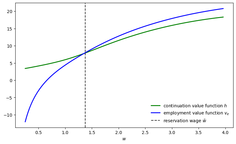
The reservation wage is at the intersection of the employment value function \(v_e\) and the continuation value function \(h\).
Here’s a function to compute it explicitly.
@jax.jit
def get_reservation_wage(model: Model) -> float:
    """
    Calculate the reservation wage for a given model.

    """
    c, α, β, ρ, ν, γ, w_grid, z_draws = model

    v_u = vfi(model)
    v_e, h = compute_solution_functions(model, v_u)

    # Compute optimal policy (acceptance indices)
    σ = v_e >= h

    # Find first index where policy indicates acceptance
    first_accept_idx = jnp.argmax(σ) # returns first True value

    # If no acceptance (all False), return infinity
    # Otherwise return the wage at the first acceptance index
    return jnp.where(jnp.any(σ), w_grid[first_accept_idx], jnp.inf)
Let’s repeat our plot, but now inserting the reservation wage.
w_bar = get_reservation_wage(model)

fig, ax = plt.subplots(figsize=(9, 5.2))
ax.plot(w_grid, h, 'g-', linewidth=2,
        label="continuation value function $h$")
ax.plot(w_grid, v_e, 'b-', linewidth=2,
        label="employment value function $v_e$")
ax.axvline(x=w_bar, color='black', linestyle='--', alpha=0.8,
           label=f'reservation wage $\\bar{{w}}$')
ax.legend(frameon=False)
ax.set_xlabel(r"$w$")
plt.show()
45.5. Simulation#
Now we run some simulations with a focus on unemployment rate.
45.5.1. Single agent dynamics#
Let’s simulate the employment path of a single agent under the optimal policy.
We need a function to update the agent’s state by one period.
def update_agent(key, status, wage, model, w_bar):
    """
    Updates an agent's employment status and current wage by one period.

    Parameters:
    - key: JAX random key
    - status: Current employment status (0 or 1)
    - wage: Current wage if employed, current offer if unemployed
    - model: Model instance
    - w_bar: Reservation wage

    """
    c, α, β, ρ, ν, γ, w_grid, z_draws = model

    # Draw new wage offer based on current wage
    key1, key2 = jax.random.split(key)
    z = jax.random.normal(key1)
    new_wage = wage**ρ * jnp.exp(ν * z)

    # Check if separation occurs (for employed workers)
    separation_occurs = jax.random.uniform(key2) < α

    # Accept if current wage meets or exceeds reservation wage
    accepts = wage >= w_bar

    # If employed: status = 1 if no separation, 0 if separation
    # If unemployed: status = 1 if accepts, 0 if rejects
    next_status = jnp.where(
        status,
        1 - separation_occurs.astype(jnp.int32),  # employed path
        accepts.astype(jnp.int32)                 # unemployed path
    )

    # If employed: wage = current if no separation, new if separation
    # If unemployed: wage = current if accepts, new if rejects
    next_wage = jnp.where(
        status,
        jnp.where(separation_occurs, new_wage, wage),  # employed path
        jnp.where(accepts, wage, new_wage)             # unemployed path
    )

    return next_status, next_wage
Here’s a function to simulate the employment path of a single agent.
def simulate_employment_path(
        model: Model,     # Model details
        w_bar: float,     # Reservation wage
        T: int = 2_000,   # Simulation length
        seed: int = 42    # Set seed for simulation
    ):
    """
    Simulate employment path for T periods starting from unemployment.

    """
    key = jax.random.PRNGKey(seed)
    c, α, β, ρ, ν, γ, w_grid, z_draws = model

    # Initial conditions: start unemployed with initial wage draw
    status = 0
    key, subkey = jax.random.split(key)
    wage = jnp.exp(jax.random.normal(subkey) * ν)

    wage_path = []
    status_path = []

    for t in range(T):
        wage_path.append(wage)
        status_path.append(status)

        key, subkey = jax.random.split(key)
        status, wage = update_agent(
            subkey, status, wage, model, w_bar
        )

    return jnp.array(wage_path), jnp.array(status_path)
Let’s create a comprehensive plot of the employment simulation:
model = create_mccall_model()
w_bar = get_reservation_wage(model)

wage_path, employment_status = simulate_employment_path(model, w_bar)

fig, (ax1, ax2, ax3) = plt.subplots(3, 1, figsize=(8, 6))

# Plot employment status
ax1.plot(employment_status, 'b-', alpha=0.7, linewidth=1)
ax1.fill_between(
    range(len(employment_status)), employment_status, alpha=0.3, color='blue'
)
ax1.set_ylabel('employment status')
ax1.set_title('Employment path (0=unemployed, 1=employed)')
ax1.set_yticks((0, 1))
ax1.set_ylim(-0.1, 1.1)

# Plot wage path with reservation wage
ax2.plot(wage_path, 'b-', alpha=0.7, linewidth=1)
ax2.axhline(y=w_bar, color='black', linestyle='--', alpha=0.8,
           label=f'Reservation wage: {w_bar:.2f}')
ax2.set_xlabel('time')
ax2.set_ylabel('wage')
ax2.set_title('Wage path (actual and offers)')
ax2.legend()

# Plot cumulative fraction of time unemployed
unemployed_indicator = (employment_status == 0).astype(int)
cumulative_unemployment = (
    jnp.cumsum(unemployed_indicator) /
    jnp.arange(1, len(employment_status) + 1)
)

ax3.plot(cumulative_unemployment, 'r-', alpha=0.8, linewidth=2)
ax3.axhline(y=jnp.mean(unemployed_indicator), color='black',
            linestyle='--', alpha=0.7,
            label=f'Final rate: {jnp.mean(unemployed_indicator):.3f}')
ax3.set_xlabel('time')
ax3.set_ylabel('cumulative unemployment rate')
ax3.set_title('Cumulative fraction of time spent unemployed')
ax3.legend()
ax3.set_ylim(0, 1)

plt.tight_layout()
plt.show()
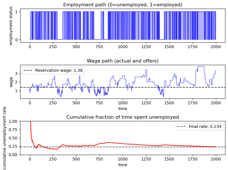
The simulation shows the agent cycling between employment and unemployment.
The agent starts unemployed and receives wage offers according to the Markov process.
When unemployed, the agent accepts offers that exceed the reservation wage.
When employed, the agent faces job separation with probability \(\alpha\) each period.
45.5.2. Cross-Sectional Analysis#
Now let’s simulate many agents simultaneously to examine the cross-sectional unemployment rate.
We first create a vectorized version of update_agent to efficiently update all agents in parallel:
# Create vectorized version of update_agent
update_agents_vmap = jax.vmap(
    update_agent, in_axes=(0, 0, 0, None, None)
)
Next we define the core simulation function, which uses lax.fori_loop to efficiently iterate many agents forward in time:
@partial(jax.jit, static_argnums=(3, 4))
def _simulate_cross_section_compiled(
        key: jnp.ndarray,
        model: Model,
        w_bar: float,
        n_agents: int,
        T: int
    ):
    """JIT-compiled core simulation loop using lax.fori_loop.
    Returns only the final employment state to save memory."""
    c, α, β, ρ, ν, γ, w_grid, z_draws = model

    # Initialize arrays
    key, subkey = jax.random.split(key)
    wages = jnp.exp(jax.random.normal(subkey, (n_agents,)) * ν)
    status = jnp.zeros(n_agents, dtype=jnp.int32)

    def update(t, loop_state):
        key, status, wages = loop_state

        # Shift loop state forwards
        key, subkey = jax.random.split(key)
        agent_keys = jax.random.split(subkey, n_agents)

        status, wages = update_agents_vmap(
            agent_keys, status, wages, model, w_bar
        )

        return key, status, wages

    # Run simulation using fori_loop
    initial_loop_state = (key, status, wages)
    final_loop_state = lax.fori_loop(0, T, update, initial_loop_state)

    # Return only final employment state
    _, final_is_employed, _ = final_loop_state
    return final_is_employed


def simulate_cross_section(
        model: Model,
        n_agents: int = 100_000,
        T: int = 200,
        seed: int = 42
    ) -> float:
    """
    Simulate employment paths for many agents and return final unemployment rate.

    Parameters:
    - model: Model instance with parameters
    - n_agents: Number of agents to simulate
    - T: Number of periods to simulate
    - seed: Random seed for reproducibility

    Returns:
    - unemployment_rate: Fraction of agents unemployed at time T
    """
    key = jax.random.PRNGKey(seed)

    # Solve for optimal reservation wage
    w_bar = get_reservation_wage(model)

    # Run JIT-compiled simulation
    final_status = _simulate_cross_section_compiled(
        key, model, w_bar, n_agents, T
    )

    # Calculate unemployment rate at final period
    unemployment_rate = 1 - jnp.mean(final_status)

    return unemployment_rate
Now let’s compare the time-average unemployment rate (from a single agent’s long simulation) with the cross-sectional unemployment rate (from many agents at a single point in time).
model = create_mccall_model()
cross_sectional_unemp = simulate_cross_section(
    model, n_agents=20_000, T=200
)

time_avg_unemp = jnp.mean(unemployed_indicator)
print(f"Time-average unemployment rate (single agent, T=2000): "
      f"{time_avg_unemp:.4f}")
print(f"Cross-sectional unemployment rate (at t=200): "
      f"{cross_sectional_unemp:.4f}")
print(f"Difference: {abs(time_avg_unemp - cross_sectional_unemp):.4f}")
Time-average unemployment rate (single agent, T=2000): 0.2335
Cross-sectional unemployment rate (at t=200): 0.2929
Difference: 0.0594
The difference above can be further reduced by increasing the simulation length for the single agent.
wage_path_long, employment_status_long = simulate_employment_path(model, w_bar, T=10_000)
unemployed_indicator_long = (employment_status_long == 0).astype(int)
time_avg_unemp_long = jnp.mean(unemployed_indicator_long)

print(f"Time-average unemployment rate (single agent, T=10000): "
      f"{time_avg_unemp_long:.4f}")
print(f"Cross-sectional unemployment rate (at t=200): "
      f"{cross_sectional_unemp:.4f}")
print(f"Difference: {abs(time_avg_unemp_long - cross_sectional_unemp):.4f}")
Time-average unemployment rate (single agent, T=10000): 0.2945
Cross-sectional unemployment rate (at t=200): 0.2929
Difference: 0.0016
45.5.3. Visualization#
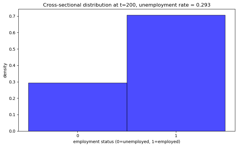
This function generates a histogram showing the distribution of employment status across many agents:
def plot_cross_sectional_unemployment(
        model: Model,            # Model instance with parameters
        t_snapshot: int = 200,   # Time for cross-sectional snapshot
        n_agents: int = 20_000   # Number of agents to simulate
    ):
    """
    Generate histogram of cross-sectional unemployment at a specific time.

    """

    # Get final employment state directly
    key = jax.random.PRNGKey(42)
    w_bar = get_reservation_wage(model)
    final_status = _simulate_cross_section_compiled(
        key, model, w_bar, n_agents, t_snapshot
    )

    # Calculate unemployment rate
    unemployment_rate = 1 - jnp.mean(final_status)

    fig, ax = plt.subplots(figsize=(8, 5))

    # Plot histogram as density (bars sum to 1)
    weights = jnp.ones_like(final_status) / len(final_status)
    ax.hist(final_status, bins=[-0.5, 0.5, 1.5],
            alpha=0.7, color='blue', edgecolor='black',
            density=True, weights=weights)

    ax.set_xlabel('employment status (0=unemployed, 1=employed)')
    ax.set_ylabel('density')
    ax.set_title(f'Cross-sectional distribution at t={t_snapshot}, ' +
                 f'unemployment rate = {unemployment_rate:.3f}')
    ax.set_xticks([0, 1])

    plt.tight_layout()
    plt.show()
Let’s plot the cross-sectional distribution:
plot_cross_sectional_unemployment(model)
45.6. Exercises#
Exercise 45.1
Use the code above to explore what happens to the reservation wage when \(c\) changes.
Solution
Here is one solution
def compute_res_wage_given_c(c):
    model = create_mccall_model(c=c)
    w_bar = get_reservation_wage(model)
    return w_bar

c_vals = jnp.linspace(0.0, 2.0, 15)
w_bar_vals = jax.vmap(compute_res_wage_given_c)(c_vals)

fig, ax = plt.subplots()
ax.set(xlabel='unemployment compensation', ylabel='reservation wage')
ax.plot(c_vals, w_bar_vals, label=r'$\bar w$ as a function of $c$')
ax.legend()
plt.show()
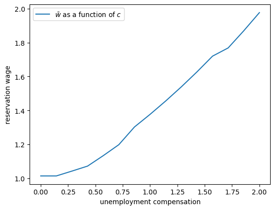
As unemployment compensation increases, the reservation wage also increases.
This makes economic sense: when the value of being unemployed rises (through higher \(c\)), workers become more selective about which job offers to accept.
Exercise 45.2
Create a plot that shows how the reservation wage changes with the risk aversion parameter \(\gamma\).
Use γ_vals = jnp.linspace(1.2, 2.5, 15) and keep all other parameters at their default values.
How do you expect the reservation wage to vary with \(\gamma\)? Why?
Solution
We compute the reservation wage for different values of the risk aversion parameter:
γ_vals = jnp.linspace(1.2, 2.5, 15)
w_bar_vec = jnp.empty_like(γ_vals)

for i, γ in enumerate(γ_vals):
    model = create_mccall_model(γ=γ)
    w_bar = get_reservation_wage(model)
    w_bar_vec = w_bar_vec.at[i].set(w_bar)

fig, ax = plt.subplots(figsize=(9, 5.2))
ax.plot(γ_vals, w_bar_vec, linewidth=2, alpha=0.6,
        label='reservation wage')
ax.legend(frameon=False)
ax.set_xlabel(r'$\gamma$')
ax.set_ylabel(r'$\bar{w}$')
ax.set_title('Reservation wage as a function of risk aversion')
plt.show()
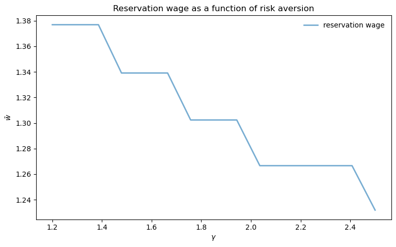
As risk aversion (\(\gamma\)) increases, the reservation wage decreases.
This occurs because more risk-averse workers place higher value on the security of employment relative to the uncertainty of continued search.
With higher \(\gamma\), the utility cost of unemployment (foregone consumption) becomes more severe, making workers more willing to accept lower wages rather than continue searching.